Building a Lock-Free Cache-Oblivious B-Tree
Part 1: Designing the Data Structure
5/6/2020
If you missed the intro, check out Part 0: A Prelude.
Research
I've spent a while scouring the internet for inspiration and found a handful of academic whitepapers to help guide me through this process:
- Cache-Oblivious Algorithms (1999)
- Cache-Oblivious Algorithms and Data Structures (2002)
- Concurrent Cache-Oblivious B-Trees (2005)
The Data Structure
The lock-free cache-oblivious B-tree structure will be made up of two parts:
- A packed-memory array that stores the raw values attached to the leaves
- A static search binary tree, used to index into a region of the packed-memory array
A packed-memory array is just a fancy way of saying a contiguous chunk of storage that has some gaps in between so we don't need to constantly reallocate it on insert or delete.
The Search Tree
To build the search tree in a cache-oblivious manner means that the nodes of the tree have to be stored in a very specific way. This is the heart of the cache-oblivious algorithm: the nodes are stored using a “van Emde Boas layout”—inspired by the van Emde Boas tree— which recursively organizes branches of the tree. As you descend deeper, you're more likely to be on a section of memory that's been cached by something, somewhere.
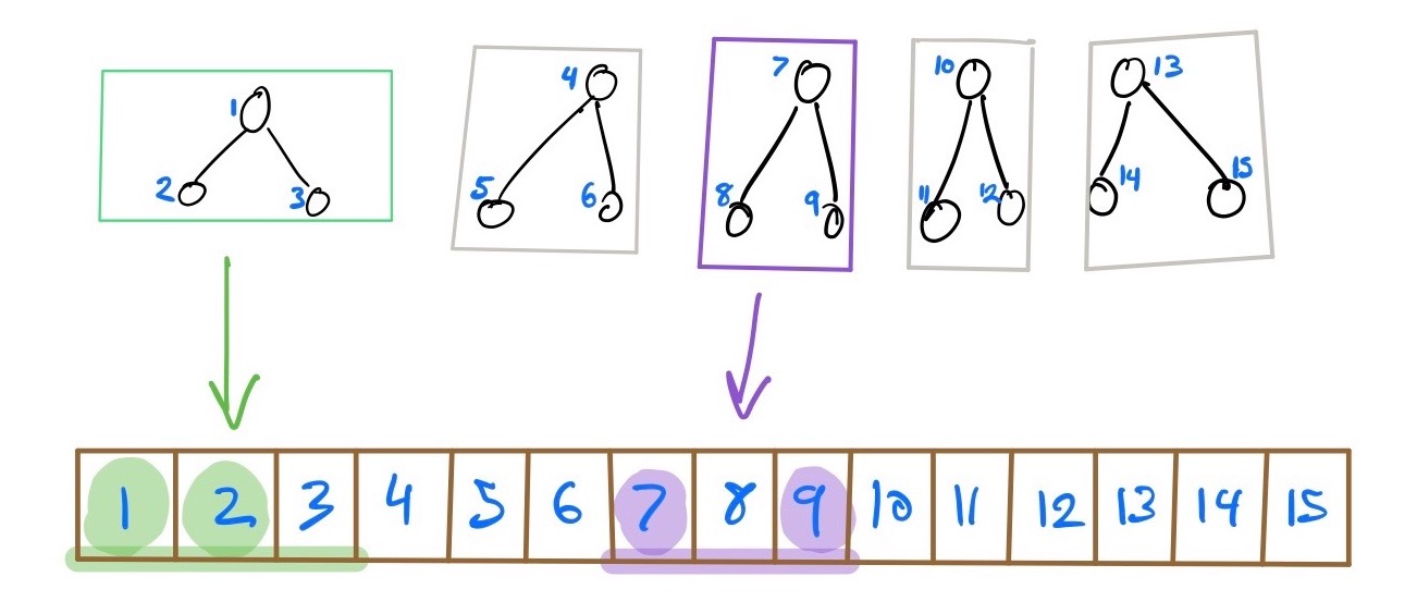
If we have a binary tree with four levels stored in a van Emde Boas layout, we end up loading a maximum of two blocks (six nodes) of the tree when performing a search:
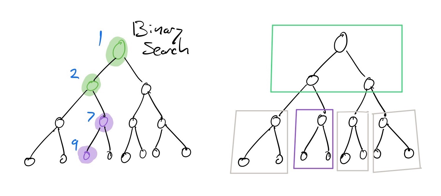
If you look at the packed memory array storing the nodes, that means we loaded two distinct ranges:
It doesn't seem particularly useful in such a small tree, but at larger scales, it could make all the difference.
As a further optimization, we let each leaf of the search tree point to a set of cells in the packed memory array. This limits the number of updates needed through the tree and allows us to deal with shifting pointers in a lock-free way. I expect that adjusting the size of this window will have an impact on concurrency performance and stale reads, but I don't quite know how to quantify it yet.
The Packed-Memory Array
The key features of the packed-memory array are:
- It is a contiguous block of data
- There are gaps to allow for insertions without reallocating
Since we also want this to be lock-free, we need to have some other clever properties:
- The packed-memory array is segmented into three; only the middle section (the active region) is populated with data
- On insertion, we can grow the active region by using the empty cells from the right
- On deletion, we can shrink the active region by giving these cells over to the left region
The real fun comes in when we try to optimize for density of the active region. This paper has a great deal of guidance on how to calculate the optimal density, but it distills down to this:
Given an active region of size N, there are log2(N) density scales. The size of your subregion determines the minimum and maximum acceptable density. If you're looking at a two-cell wide window, it might be okay to be 100% full. If you're looking at the entire packed-memory array, you might want it to only be a maximum of 1/2 full. As you move through the scales, there are min- and max- density values that let you know if you should reclaim this space or redistribute elements to make more room.
Time for Some Math
Now that we conceptually (kinda) know what we're dealing with, let's put pen to paper and figure out (a) how much storage we need to allocate and (b) how to lay it all out.
Computing the Packed-Memory Array
Let's work through the equations following a few definitions:
- For a subarray of size
n,i =log2(n)- e.g. for
[_; 32],i = log2(32) = 5
- e.g. for
Tiis the maximum allowed density foriPiis the minimum allowed density fori- The maximum density we want to allow of the entire active region is
Tmin - The minimum density we want to allow of the entire active region is
Pmax
Caveat: I am not a comp-sci major nor a math major, and my understanding of these equations might be completely wrong.
Time to make some decisions. Let's say that at any given time, we want the active region to be at most 1/2 full, and at minimum 1/4 full:
Tmin = 1/2Pmax = 1/4
From those constant values, we can deduce the "ideal density" of the entire packed-memory array (including the empty regions):
d = (Tmin – Pmax) / 2 = 1/8
To figure out how big we need to make our entire packed memory array (including those two empty regions), we can do some simple math. Let's say we want to store N=30 elements:
m = N / d = 240
Now we know we need to allocate an array of length m to store all of our values without the result being too dense.
I'm not sure if it's necessary (once we get to coding, we'll find out!), but I've found it much easier to reason about these numbers when working with double-exponential power-of-two sized arrays. The closest to 240 is m = 223 (256 slots).
Computing the Search Tree
As mentioned earlier, each leaf of the tree points to some amount of cells in the packed memory array. This was casually mentioned in one of the above papers, but I expect this formula is something we can tweak. For now, let's go with it:
slots = log2(m) = 8
Each leaf in our tree will point to a block that is 8 slots in length. From there, we can calculate the number of leaves required:
leaves = m / slots = 32
Since this is just a binary tree, we can compute the total number of nodes required to represent the tree from just the number of leaves:
nodes = 2 × leaves – 1 = 63
Laying out the Tree
After running through the above, we've determined the following:
- Our packed-memory array (that will store the values) needs to be 256 cells long
- Our search tree has 63 nodes
Now that the icky math is over, we get to the fun part! We need to figure out the layout for storage (okay there's still some icky math left). The first step is to compute the height of the tree:
tree_height = log2(nodes + 1) = 6
Binary trees don't usually include the root node in their height, but in the papers I've read for cache-oblivious trees, they all seem to, so we're just going to go with it.
Once we've got the tree height, we want to divide the tree roughly in half, ensuring the lower half is a power-of-two, even if the top half isn't. If the lower half is a power of two, we can ensure our recursive partitioning will split nicely as we descend down (where there will be exponentially more branches than in the upper half).
lower_height = ceil(tree_height / 2) = 3
Since 3 isn't a power-of-two, the closest useable value for lower_height is 4. That means the upper subtree has to have a height of whatever remains:
upper_height = tree_height – lower_height = 2
Now that we have that math down, we have to repeat it recursively for each subtree, starting with the upper subtree.
This illustration has each node numbered in the order inserted:
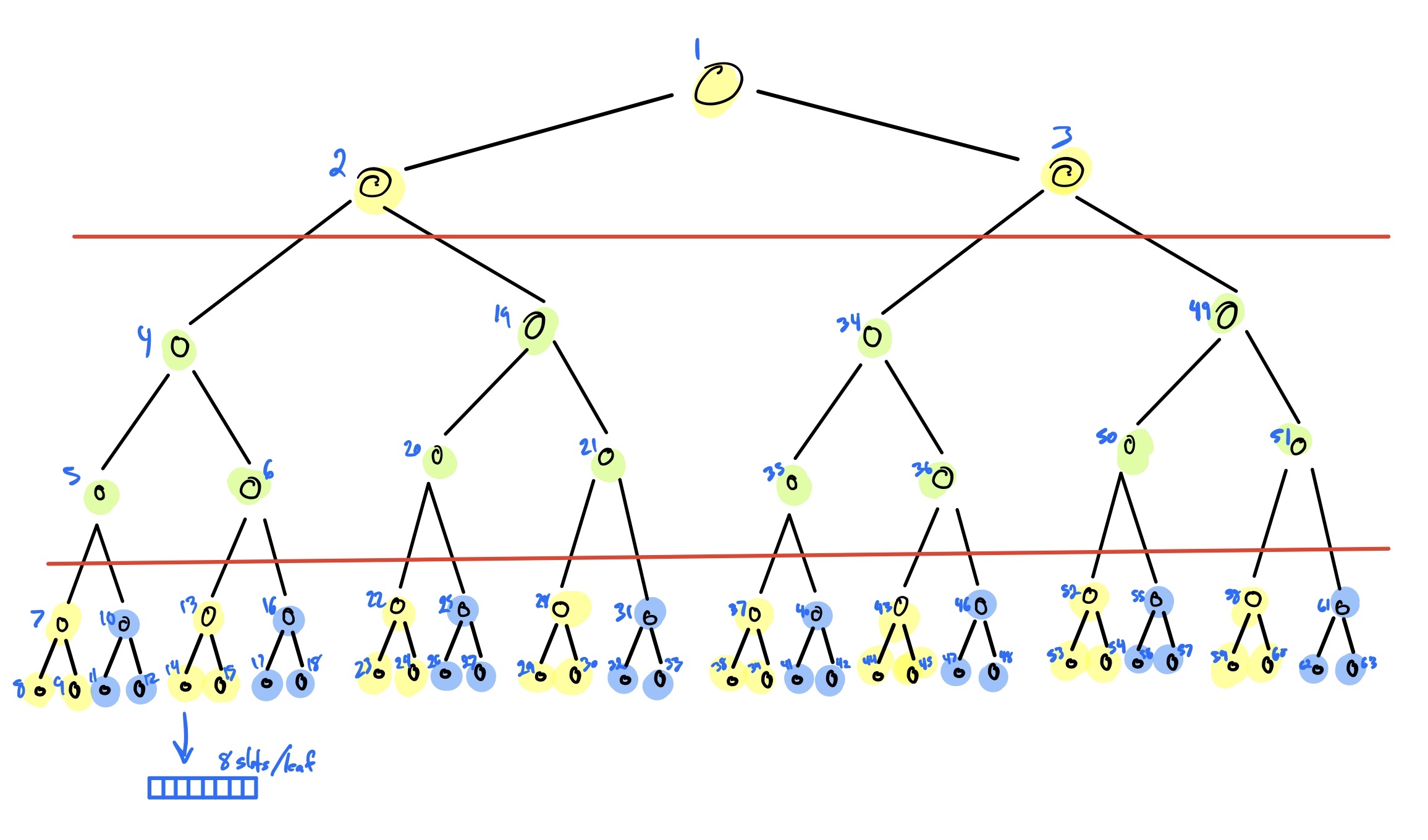
The first red line shows our initial cut, with the upper subtree having a height of 2 and the lower subtrees a height of 4. Since we cannot divide the upper subtree any further, we are free to lay it out from root-to-leaf in slots 1-3.
Now we are left with four branches, each with a height of 4. Applying the layout equation above gives us an upper subtree height of 2 and a lower subtree height of 2, as shown by the second red line. Once again, we can't divide any further, so we can proceed to lay out the branches in storage, beginning with the upper subtree (slots 4–6).
That's all the theory I understand up until this point. Next post we'll begin taking a look at how to actually implement this in code.